The economics and politics of income distribution:
How society divides its wealth amongst its members is at the core of economics (and politics). It is generally taken for granted that more equal distributions are, ceteris paribus, more desirable for society. (This is also a natural corollary given dimishing marginal utility in consumption/income and if society cares about each of its members equally.) However, there is a debate on what trade-offs may exist between degrees of income distribution and other goals of society (e.g. economic growth).
Emmanuel Saez (UC Berkeley) and Thomas Piketty (Paris School of Economics) are two leading researchers of income inequality, with a focus on the United States (and France), where growing income inequality since the late 1970s (coincident with the deregulation of markets) has made that country the most highly unequal of all industrialised nations. (The Gini coefficient (see two items below) of the United States was 46.8 in 2009 (48.9 in 2007, Congressional Budget Office (CBO) estimate); for comparison, it was 32.1 in Canada and 32.7 in France in the same year.) Aside from the Gini measure of income inequality, one of the most illutsrative indicator of growing American inequality — which is also reflected in many other industrialised nations — is the growing share of income (wealth) earned (amassed) by the top 1 percent of the population. The richest 1 percent of Americans own about half of the wealth in the United States and their share of national income exceeds 20 percent. Another common yardstick used to demonstrate the growing gap between the rich and the masses is the pay package of CEOs compared with the average worker. In the United States, CEOs of large publicly traded companies earn a multiple of about 500x that of the median worker, while a recent Canadian study (Recession-proof: Canada’s 100 best paid CEOs) pegged the ratio in Canada at 155x. Miles Corak of the University of Ottawa maintains a great blog on socio-economic matters (children, education, immigration, inequality & poverty, occupy Wall Street, and unemployment): Economics for public policy.
(Saez and Piketty, along with Facundo Alvaredo (Paris School of Economics) and Tony Atkinson (Oxford University) maintain a great website that is a database for world income distributions: The world top incomes database. For those interested in a good collection of articles and debates on the topic the New York Times has a dedicated page for the topic of inequality: The Great Divide.)
It is argued that a rise in income inequality is a natural phenomenon of economic growth for countries in the earlier stages of development. This theory says that income inequality follows a Kuznet curve — i.e. it grows as national income initially rises, then falls thereafter as national income reaches a certain level. Nevertheless, this notion of the welfare state being a “normal good” is being challenged by the growth in inequality in rich countries since the 1980s: Top incomes in the long run of history (Atkinson, Piketty, and Saez (2010)).
A polarisation of incomes comingled with populations dividing along the lines of education and ethnicity will strain social cohesion, especially in diverse societies. Although Toronto is often held up as a paragon of a diverse city that works (though such claims are now hotly contested), a phenomenon of sorting has taken place and continues to transpire in the city: Economic inequality in Toronto. How countries–and especially cities where the trend is most acute–deal with the growing gap between the wealthy and everyone else will be one of the great challenges of the 21st century for policy makers.

Income beta:
Economists measure the persistence of income across generations with the so-called “income beta”, i.e. the coefficient in the regression of an offspring’s income on parental income. A coefficient of 1 implies that a child’s income is perfectly predictable by its parents’ income, while a value of zero implies that parental income has no relation to a that of a child’s. It has been argued that a country like the US tolerates a higher level of inequality (vis-à-vis other industrialised countries) because it offers more opportunity for social mobility (i.e. income betas are low). However, much of the academic evidence points at a different reaility. The seminal contribution to this debate was from Nancy Stokey who wrote a paper in 1996 (Shirtsleeves to shirtsleeves: The economics of social mobility) that essentiallly debunked the myth of American social mobility, showing that income mobility in the US was lower than that of many European countries (contradicting a priori beliefs), as well as that of Canada.
Relative versus absolute income mobility:
According to one recent study (Jantti et al (2006): “American exceptionalism in a new light”), 42 percent of American men born into the bottom quintile of the income distribution stay in the bottom quintile as adults; whereas 8 percent of American men born into the lowest income quintile go on to the top quintile as adults. In the UK–a country where class matters — 30 percent of men born into the bottom quintile remained in the bottom quintile as adults. A larger variation in US incomes naturally result in less relative income mobility in the US vis-à-vis more equitable countries. That is, since the absolute gap from the bottom to the top quintile is higher in the US this naturally limits the number of people moving from one quintile to another compared with countries where the income bands are more tight. Absolute income mobility, on the other hand, measures a child’s income relative to parental income, rather than a child’s position in the income distribution. By this metric The Pew Research Centre reckons that over 80 percent of Americans have higher (real) incomes than their parents (but largely because of a growing economy). There is thus a debate on which of the metrics of mobility are more relevant for policymakers.
The below chart from Miles Corak (University of Ottawa) shows the Gini coefficient on the x-axis and intergenerational earnings elasticity (i.e. income stickiness) on the y-axis. Denmark, Norway, Finland and Canada have high levels of income mobility, whereas South Africa, Peru, China and Brazil have little income mobility. Inequality can be deemed tolerable if there is significant mobility. The graph below shows that inequality is accompanied with less mobility.

Gini coefficient:
One of the most widely known measures of inequality is the Gini coefficient, named after academic Corrado Gini (University of Bologna) who developed the simple (first-order) measure of distribution. It is calculated by rank-ordering a population by the distribution variable along the x-axis and the cumulative value of the distribution variable along the y-axis–for clarity let the distribution variable be income. (This then is the Lorenz Curve, named after economist Max O. Lorenz.) Both the x-axis and the y-axis are normalised to 1 so that the diagonal line from the origin (0,0) to the point (1,1) represents a perfectly equal income distribution (i.e. the nth percentile of the population accounts for n percent of total income). The Gini coefficient is thus the area between the diagonal and the cumulative income line; to express it as a measure from zero to one it is multiplied by two. (It is often also expressed as number between 0 and 100.) A Gini coefficient of zero implies that the cumulative income line is identical to the diagonal line, so that income is perfectly equally distributed. In the case where all but the top person earns zero (i.e. the top person earns all of the income) the cumulative income line would be a horizontal line along the x-axis and jumps to (1,1) at the last (and richest) person. Here the Gini is 1 and is the most unequal possible outcome of income distribution. Of the 135 countries where data is available, the nation with the lowest Gini coefficient is Sweden (23.0) while the highest level of income inequality is found in Namibia (70.7); the median country in the list is Mauritius (39.0). The per capita GDP of Sweden, Namibia and Mauritius are $61,098, $6,087 and $8,520, respectively (IMF estimates).
Income / wealth inequality in Canada the United States:
There has been some debate on the linkage between tax rates and income inequality. Namely, that a rise in the share of income earned by the upper end of the income distribution has been a result of a decrease in the top personal marginal tax rate. This supposes that higher incomes are a result of transfers of income from the corporate to personal sectors as taxes have eased on personal income. In the US the top marginal tax rate on income has steadily declined from over 80 percent in the 1960s to its current level of 35 percent, whereas the drop in the top marginal tax rate in Canada over the same period has been much more modest. Using these two different paths in the tax rate, and utilising the fact that both countries displayed sharp increases in the earnings of the top one precent, Emmanuel Saez and Michael Vaell show in a 2004 AER paper (The evolution of high incomes in North America: Lessons from the Canadian experience) that rising income inequality in the US has not been merely a consequence of a shifting of the tax base in response to a lowering of personal tax rates.
The growing polarisation of incomes in the United States (see, e.g. Income inequality in the United States, 1913-1998 (Piketty and Saez (2003)) has garrered a lot of public attention; however, the phenomenon of rising income inequality has also been happening at a similar magnitude in Canada (see, e.g. The rise of Canada’s richest 1%). Nevertheless, the US remains the focal point for this line of study because inequality there is the highest amongst rich nations, and it is the highest it has been since the Gilded Ages, just before the Great Depression spawned redistributive economic policies (the New Deal). The parallels in the current economic environment are thus uncanny, with some arguing that there may be a causal relationship between inequality and economic depressions.
Wealth inequality is typically more extreme than income inequality. For example, in the United States the richest 1 percent of income earners claim a share of national income of 23%, whereas the wealthiest 1 percent own 50 percent US wealth. In Canada the top 1 percent of income earners account for 18 percent of national income, while the wealthiest 1 percent control 30 percent of national wealth.
Defining the poor and the rich:
There is no formal definition for when an individual or household is considered “poor” or “rich” (although in a 2011 survey by Gallup the median response cited by Americans as rich was an annual income of $150 thousand). Some countries define the poverty line using a marker relative to median income (e.g. the poverty line is defined as half the median income in many European countries), while an absolute measure for poverty is used in North America (which is typically specific to a given area to account for cost-of-living differences), and in some developing countries poverty is defined by caloric intake.
An analogue to the European view of poverty would be to define the rich as those with earnings exceeding a certain multiple of median income–a marker on the order of 5x or 10x median income might thus be appropriate. Using US data (median household income of about $50 thousand) this suggests that, at a ratio of 5x, the rich are those households with incomes in excess of $250 thousand, or $500 thousand if the 10x multiple is used instead. On the other hand, an absolute cut-off to define rich depends on the perspective of who you ask, as the Gallup poll mentioned in the preceding paragraph shows that the number varies according to the respondents own level (i.e. reference point) of income. (In any case, the absolute figure of $150 thousand is a multiple of 3x of median income, and $1 million would be a multiple of 20x of median income.) One can also define the rich (in terms of income) as those in the top x-percentile of the income distribution, where x in the Occupy Wall Street (OWS) movement has become 1 (i.e. the rich are those in the top 1 percentile of the income distribution). Using US data this would imply a household income threshold (gross, before tax) of US$ 350 thousand in the US (a 7x multiple of median income) using IRS data from 2011 — other data suggests that the top 1 percent threshold is much higher (on the order or $500 thousand). In Canada, where taxpayers file as individuals, the cut-off to the top 1 percentile of the income distribution would require an annual income of C$170 thousand.
Defining the rich would have interesting policy implications because of the political push to “tax the rich” to help countries restore their financial position, and the because of the growing concern that high levels of inequality may be deleterious to the greater society. Data also show that it has been the already-rich who have captured most of the economic gains since the 1980s. Defining the top marginal tax rates — i.e. those that would apply only to the “rich” — relative to median income is one possible step in the right direction to deal with the growing gap while being incentive compatible. That is, if the top tax rates are a (positive) function of the median income of a country (e.g. the top tax rate kicks in at 5x of median income), then the rich (the 1 percent or so) — who are the ones with the political power to make meaningful policy changes – can increase their after-tax income by either raising their own pre-tax income and/or by raisig the national median income. Similarly, a CEO’s pay could be set as function of the median income of the country, in addition to the company’s financial performance (e.g. compensation is capped at 50x of national median income or 50x a weighted average of the national and firm median incomes). Under this scheme, CEOs — who can sway not just the direction of their companies, but also of national policies — are incentivised to work for the betterment of the company, workers, and society as a whole. (See: “A fairer pay system?“)
Non-linearity of income/wealth distribution (in progress):
A point that has caught the public’s attention in the debate on income distribution is the gap between the richest 1 percent and the rest of society. Often the richest 1 percent (either measured by income or wealth) is taken synonomously with the “rich”, yet even within this group there are large variations in their composition (occupation, power, etc.) and their outcomes (i.e. level of income). Those that belong to the top 99.0 to 99.5 percentile have very different characteristics than those in the top 99.9 percentile. Indeed, the lion’s share of the growth in the income and wealth of the top 1 percent of the population in Canada and the USA have accrued to the top 0.1 percent.
Social welfare function:
Economists use so-called social welfare functions (SWF) to rank the outcomes of social states. More precisely, it is a function that assigns a real number to a set of possible states of the world (i.e. a distribution of consumption and leisure possibilities), where higher numbers are associated with higher (ordinal) levels of social utility. A SWF can thus be used to assess the desirability of alternative social states. Whence the SWF is derived is contentious as there are many ways to aggregate individual utilities into a social utility, whose merits depend on one’s political beliefs. A few examples of SWFs include: (i) a utilitarian SWF (maximises the sum of the utilities); (ii) a maxi-min SWF (maximises the utility of the lowest person); (iii) a maxi-max SWF (maximises the utility of the highest person); (iv) a maxi-med SWF (maximises the utility of the median person). In more concrete terms, economics Nobel laureate (1998) Amartya Sen proposed that policy makers try to maximise a utility function of the form: (per capita GDP) × (1 − Gini coefficient).
Pareto efficiency / optimality:
An economic distribution / outcome is said to be Pareto efficient (or Pareto optimal) if any redistribution necessarily makes at least one person worse off. Said another way, a change in an outcome is said to be Pareto improving if it makes at least one person better off without making anyone worse off. If people’s utility’s are purely determined by their own consumption patterns, then a change in income distribution whereby the incomes of the richest one percent grows by 275 percent, while the incomes of the 81st through 99th, 21st through 80th, and bottom 20th percentiles grow by 65, 40 and 18 percent, respectively, is Pareto improving. In this case, the richest one percent claims 60 percent of all income growth while the bottom 90 percent drives 8.6 percent of growth. (This was the case in the United States when comparing real income change from 1979 to 2007. See the CBO report: Trends in the distribution of household income between 1979 and 2007.) However, Pareto efficiency is neither necessarily fair nor socially optimal. The controversy surrounding growing income inequality, which has spawned, amongst other things, the Occupy Wall Street (OWS) movement of 2011, is a testament to the social dissatisfaction (at least by some) of the growing income gap.
Does inequality matter?
It is generally reported that lower levels of inequality are associated with higher levels of social satisfaction: Across studies and surveys, people report a greater sense of personal satisfaction with lower levels of income inequality. However, lower levels of inequality, per se, do not positively impact the consumption possibilities of households, so standard economic theory does not have an avenue for direct benefits from an egalitarian society. Nevertheless, with diminishing marginal utility of income, there are definite societal-level benefits to more equitable distributions under any social welfare function that weighs the utilities of individuals in society in more or less equal ways.
It is generally assumed that the welfare function of individuals consists of a composite good, as well as from leisure. Standard theory does not incorporate jealousy or altruism as factors that affect the felicity of individuals. Notwithstanding that, a SWF is not merely the sum of the utilities of the group (although this may be the case under a utilitarian SWF), so it may also include a level of income inequality as a direct argument. Whether inequality matters on a social-utility level depends on the goals of society. However, if higher levels of inequality are, per se, disruptive to the market and lead to unstable paths for the economy there are real reasons to be concerned about how to divide the pie. This is exactly the case for those that propose that high levels of inequality may trigger economic depressions.
Rawls’s veil of ignorance:
John Rawls, a Harvard philosopher who was educated at Princeton and Oxford, provides one of the most celebrated intellectual underpinnings for a society that is more equitably distributed in his masterpiece, “A theory of jutsice” (1971), which is at the foundation of liberalism. (Rawls’s intellectual opposite was Nozick, a colleague at Harvard, who argued in favour of libertarian justice in his work, “Anarchy, state, and utopia” (1974).) In Rawls’s intellectual search for a definition of a just society, he considered two socities: One in which the variation in outcomes between the best and worst are high, versus one in which the dispersion in outcomes are low. He argued that the more just society is one which a person would choose ex-ante if he did not know his relative position. A natural predisposition for risk aversion in humans thus led him to conclude that a more equitable distribution was a society which is more fair, so that economic, political, and social institutions should support outcomes that look more kindly on the less well-off.
Redistribution of income:
Because money is fungible and transferable it is often targeted for redistribution. It is seldom that other outcomes (athletics, beauty, health, etc.) are redistributed, with the exception of placements into higher education (c.f. the debate on affirmative action policies that redistribute spots in higher educational institutions). Taxes and transfers are the primary ways to effect income redistribution. Because taxes are distortionary they elicit strong responses, even if the purpose of the tax, or where the tax earnings are earmarked for, are laudable. Whether such redistributions are “fair” or necessary are highly contentious and one of the wedges that divide the political left and right. Even Rawls’s veil of ignorance is agnostic on this point as he only contends that ex-ante a more equitably distributed society is fair, but does not take a position on ex-post transfers of income once the distribution has been realised. With transfers from one individual to another there is no (Pareto) efficient solution since any transfer of income necessarily reduces the consumption possibilities of the donor. (Though this may be a socially optimal transfer, especially if the donor is benevolent and derives utility from charity.)
Optimal taxation policy (WIP):
The tax rate that maximises government revenue (restricted in this discussion to income tax) is the so-called “optimal tax rate”. This rate (between 0 and 100 percent) is thought to be increasing in the tax rate at low levels of taxation and decreasing at high levels, was infamously described by economist Arthur Laffer in 1974 on a back of aserviette (although Laffer makes no claim of inventing the concept itself), which became a big argument of the conservative tax-cutting movement in the 1980s in countries such as the UK and the USA. Indeed, the curve that illustrates the elasticity of tax revenues as a function of the tax rate now bears the name of Arthur Laffer: The Laffer Curve. This figure is merely the rate that maximises tax revenues, and makes no normative statements about the fairness of the tax rate or how the taxes are spent. Much debate has ensued about the appropriate top marginal tax rate as countries deal with growing income inequality and public. This has been more than just an academic subject in a country such as France where the top marginal tax rate was set at 75 percent, a platform on which Francois Hollande campaigned successfully on to oust the incumbent, Nicolas Sarkozy, in 2012. In an op-ed in The Guardian, Saez and Piketty (2013) argue that the top marginal rate could be set as high as 80 percent: Why the top 1% should pay tax at 80%. How the incentive to work responds to the effective wage (i.e. after-tax income) is ambiguous since the income and substitution effects work in the opposite direction — a higher wage induces people to consume more leisure (a normal good), but at the same time a higher wage makes the relative price of leisure more dear, so that it is consumed less.
Assortive mating (WIP):
Assortive mating refers to the fact that
Distribution of income by race/ethnicity (WIP):
Income and ethnicity/race are highly correlated in multicultural/multiracial societies (and also across countries). In the United States the median household income by race
Case study 1 (Singapore, 2013):
Singapore is one of the 20th century’s great development success stories. In 1965 — the year it was expelled from Malaysia — it had a per capita GDP not much more than $500. With limited geography, no natural resources and hostile neighbours its fate was, at best, murky. But by 2013 it had transformed itself into one of the world’s alpha cities, with the fourth largest financial centre and amongst the five busiest container ports. Its per capita GDP had grown to $55 thousand, ranking it amongst the world’s richest countries. However, its development has not been without challenges, most notably the city state has a high level of income (and wealth) inequality. The below are charts of the income inequality in Singapore based on 2013 tax filings. (Data note: Those earning less than SGD 20,000 (annual) are excluded from paying taxes in Singapore.)
Income is a variable that is log-normally distributed. This means that its distribution is bounded below (at zero) and is skewed. (In mathematical terms, the logarithm of the distribution is normally distributed.) The below is a histogram of income in Singapore (2013), which takes on the log-normal shape.
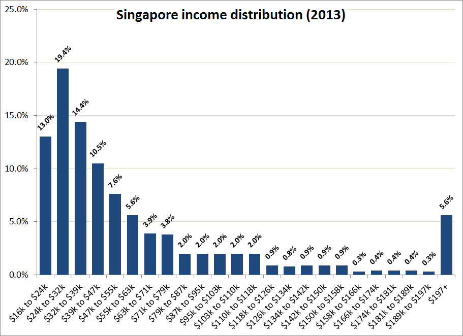 Source: http://www.salary.sg/2013/compare-your-annual-income-2013/
The CIA Factbook reports Singapore’s Gini coefficient (2013) as 46.3. This ranks the country as one of the more inequitable countries amongst developed economies. The below is a chart of the Lorenz Curve and the estimated Gini coefficient based on 2013 tax filing data. The Gini calculated (0.51) is higher than that reported in the CIA Factbook. This could be because the below chart is based on incomes before taxes and redistribution. Nevertheless, with a Gini even higher than the United States, Singapore’s rapid ascension into a global financial powerhouse seems to have lifted all boats, but not evenly. Although such a transformation may be Pareto efficient, such uneven growth may engender social unrest.
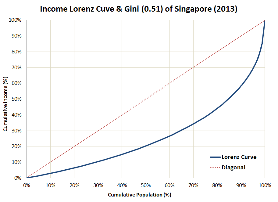 Source: http://www.salary.sg/2013/compare-your-annual-income-2013/
Median income in Singapore is just shy of $42k, while the minimum threshold into its top-1 percent is $500k. This gives a ratio (top-1 percent to median) of almost 12x. For comparison, the median income in the United States is $39k (for those working full time, between the ages of 24 and 65, which is the natural comparison to the Singapore data since the Singapore data is truncated below at SGD 20k), while entry into its top-1 percent is $394k. The US ratio — which is already high amongst developed nations — is 10x; i.e. below that of Singapore.
Of course, the proper comparison is not Singapore versus USA, but rather Singapore vs New York City. According to a CUNY study (Bergad, 2014) the household income Gini for New York City in 2010 was 0.50 — suggesting that the current level may be higher given a secular trend that has seen the Gini level rise from 0.44 in 1990 to 0.49 in in 2000 and 0.50 in 2010. Levels of income inequality are higher in urban centres versus rural (or suburban) areas; but whether national (blended) levels are higher versus the urban level is not clear.
Case study 2 (New York City):
WIP
References:
- Bergad, Laird W. (2014): “The concentration of wealth in New York City: Changes in the structure of household income by race/ethnic groups and Latino nationalities 1990-201).” Latino Data Project – Report 56, Graduate Centre CUNY, January 2014.
- Rawls, John (1971): “A theory of justice.” Cambridge, USA: Belknap Press.
- Weinberg, Danile H. (2011): “US neighbourhood income inequality in the 2005-2009 period.” American Community Service Reports, US Census Bureau, October 2011.